Analyzing OPEC Member Crude Oil Production Quotas

Will Rodman | Data Science | Tulane University

Project Link: https://willcrodman.github.io

Introduction

This project dives into data about OPEC (Organization of the Petroleum Exporting Countries) crude oil production and OECD (Organization for Economic Co-operation and Development) countries from 1960 to 2022. Including providing political context of OPEC and OECD, exploring their respective roles and significance in the global oil trade. The data source for this project is from the official OPEC website, which includes data such as crude oil production, demand, spot prices, refinery throughput, refinery capacity, and OPEC production quotas by country.

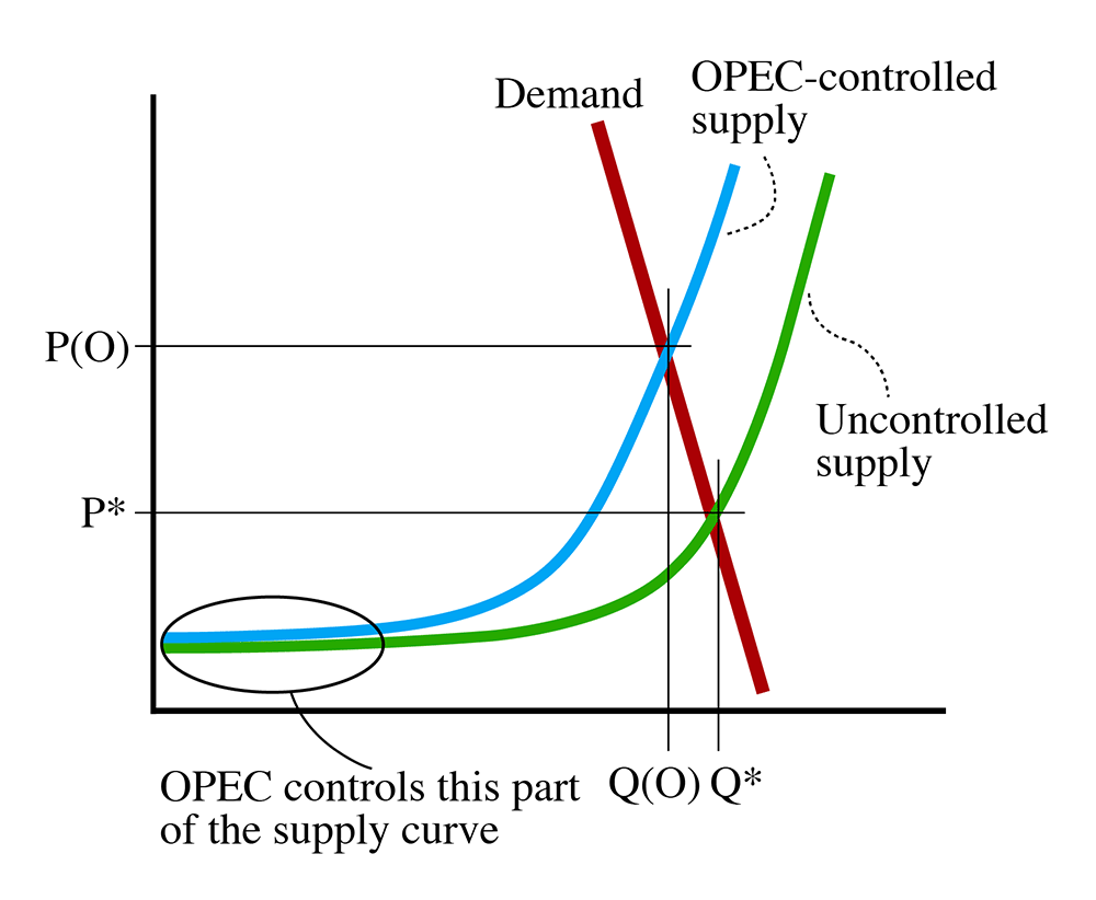
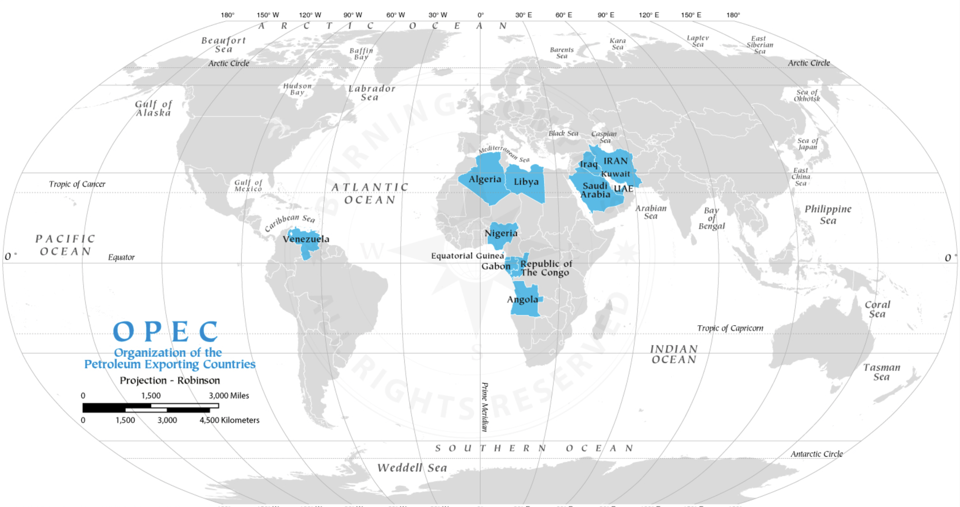
Founded in 1960, OPEC comprises a group of petroleum-exporting nations. OPEC was created with the primary aim of asserting collective control over their oil resources and global oil trade. OPEC's founding members included Iran, Iraq, Kuwait, Saudi Arabia, and Venezuela. Over the years, the organization has expanded to include several other member nations, totaling 13.

It is important to focus on OPEC member nations due to their global importance as petroleum exporters. Alongside OECD countries, who are reliant on oil imports to meet their energy needs, and have historically been affected by changes in OPEC production quotas and embargoes. This by fixing production and suppliers, OPECs behaves like as cartel-style supplier.

Data Source: https://asb.opec.org/data/ASB_Data.php

# Installing library requirements.
!pip install pandas numpy scipy matplotlib sklearn --quiet

DEPRECATION: Configuring installation scheme with distutils config files is deprecated and will no longer work in the near future. If you are using a Homebrew or Linuxbrew Python, please see discussion at https://github.com/Homebrew/homebrew-core/issues/76621
DEPRECATION: Configuring installation scheme with distutils config files is deprecated and will no longer work in the near future. If you are using a Homebrew or Linuxbrew Python, please see discussion at https://github.com/Homebrew/homebrew-core/issues/76621
WARNING: There was an error checking the latest version of pip.

# Import library requirements.
import pandas as pd
import warnings
import numpy as np
import matplotlib.pyplot as plt
from scipy.stats import zscore
import re
from pandas.plotting import scatter_matrix

from sklearn.ensemble import RandomForestRegressor
from sklearn.model_selection import train_test_split
from sklearn.metrics import mean_absolute_error
from sklearn.impute import SimpleImputer
from sklearn.metrics import precision_score, recall_score

warnings.simplefilter(action='ignore', category=FutureWarning)

OPEC and OCED Organizations

While OPEC consists of major oil-producing nations such as Saudi Arabia, Iran, Iraq, and Venezuela, among others. OECD comprises economically advanced nations, primarily in Europe and North America, which heavily rely on oil imports to fulfill their energy requirements. Currently there are 38 member countries in OECD including the United States and United Kingdom.

The primary difference between OPEC and free market nation in OECD is how OPEC acts as a cartel-style supplier. In economics, a cartel supplier is defined "a formal agreement between a group of producers of a good or service to control supply or to regulate or manipulate prices" (investopedia.com).

# List of OPEC countries in 2023. 
opec_countries = pd.read_csv('data/countries/opec.csv', header=None, squeeze=True)
opec_countries.head(13)

0                  Algeria
1                   Angola
2        Equatorial Guinea
3                    Gabon
4                 I.R.Iran
5                     Iraq
6                   Kuwait
7                    Libya
8                  Nigeria
9                    Congo
10            Saudi Arabia
11    United Arab Emirates
12               Venezuela
Name: 0, dtype: object

# List of OECD countries in 2023. 
oecd_countries = pd.read_csv('data/countries/oecd.csv', header=None, squeeze=True)
oecd_countries.head()

0    Australia
1      Austria
2      Belgium
3       Canada
4        Chile
Name: 0, dtype: object

Crude Oil Production and Demand

Extract, Transform, and Load (ETL) Data

This imports crude oil production and demand for countries world wide (including all OPEC members) from 1960 to 2020. Crude Oil refers to the fossil fuel that exits in Earths geological formations. They will be stored in the project as Pandas DataFrames, along with a third DataFrame that describes countries domestic crude oil demand deficits per year.

$\text{Deficit}_{\text{year}} = \text{Production}_{\text{year}} - \text{Consumption}_{\text{year}}$

# Importing oil production dataset.
oil_production_df = pd.read_csv("data/opec_upstream/world_oil_production.csv", index_col="Index")
oil_production_df.replace('na', np.nan, inplace=True)
oil_production_df = oil_production_df.astype(float)

# Replacing incorrectly labeled countries. 
replace = {'IR Iran': 'I.R.Iran', 'Saudi Arabia1': 'Saudi Arabia', 'Kuwait1': 'Kuwait', 'Syrian Arab Rep.': 'Syria', 'Uzbekistan`': 'Uzbekistan'}
oil_production_df = oil_production_df.rename(index=replace)

# Importing oil demand dataset. 
oil_demand_df = pd.read_csv("data/opec_downstream/world_oil_demand.csv", index_col="Index")
oil_demand_df.replace('na', np.nan, inplace=True)
oil_demand_df = oil_demand_df.astype(float)

# Merging oil production and oil demand datasets; One-to-one matching needed to compute oil deficit. 
oil_deficit_df = oil_demand_df.merge(oil_production_df, left_index=True, right_index=True, how='inner')

# Iterating over years of oil production and oil demand to compute oil deficit. 
for year in range(1960, 2023):
    year_x, year_y = f"{year}_x", f"{year}_y"
    oil_deficit_df[year] = oil_deficit_df[year_x] - oil_deficit_df[year_y]
    oil_deficit_df = oil_deficit_df.drop(columns=[year_x, year_y])
    
# Transposing DataFrames to set years as index.  
oil_production_df = oil_production_df.transpose()
oil_demand_df = oil_demand_df.transpose()
oil_deficit_df = oil_deficit_df.transpose()

# Converting year index to datetime object. 
oil_production_df.index = pd.to_datetime(oil_production_df.index, format='%Y')
oil_demand_df.index = pd.to_datetime(oil_demand_df.index, format='%Y')
oil_deficit_df.index = pd.to_datetime(oil_deficit_df.index, format='%Y')

# Display DataFrame
oil_deficit_df.head() 

Index	Canada	Chile	Mexico	United States	United Kingdom	Australia	China	India	Indonesia	Malaysia	...	Egypt	Equatorial Guinea	Gabon	Libya	Nigeria	Russia	Azerbaijan	Kazakhstan	OPEC	OECD
1960-01-01	290.164	24.395	-181.090	3189.7	918.239	269.000	105.50	143.806	-309.6	9.0	...	37.684	0.0	-12.4	4.0	-1.4	-1010.1	NaN	-4.1	-7773.752195	7966.45244
1961-01-01	213.230	23.284	-181.544	3213.1	969.721	287.000	100.85	153.615	-313.3	16.0	...	28.730	0.0	-11.9	-14.2	-27.0	-1214.3	NaN	-5.8	-8407.232041	8562.18744
1962-01-01	194.771	20.082	-181.161	3522.0	1063.617	297.000	96.55	138.397	-328.4	22.0	...	13.908	0.0	-13.4	-176.3	-50.5	-1398.8	NaN	-7.4	-9527.366548	9691.92063
1963-01-01	213.598	19.499	-154.292	3947.3	1155.410	336.000	120.15	143.370	-315.0	29.0	...	-1.710	0.0	-13.7	-435.8	-54.5	-1488.7	NaN	-7.2	-10522.296582	11105.58335
1964-01-01	234.151	21.190	-120.369	4106.7	1276.202	349.163	138.35	131.591	-318.6	36.0	...	-14.546	0.0	-17.0	-855.4	-96.2	-1671.7	NaN	1.7	-11910.261359	12455.20195

5 rows × 37 columns

Because our two datasets do not have a perfect one-to-one matching, deficits cannot be computed for every country. This mean exploratory data analysis will be for all OPEC member countries and a limited number of OECD member countries. In addition here are the missing years for each country.

print('Countries in oil production DataFrame:', len(oil_production_df.columns))
print('Countries in oil demand DataFrame:', len(oil_demand_df.columns))
print('Countries in oil deficit DataFrame:', len(oil_deficit_df.columns))
oil_deficit_df.isna().sum()

Countries in oil production DataFrame: 48
Countries in oil demand DataFrame: 61
Countries in oil deficit DataFrame: 37

Index
Canada                   0
Chile                    0
Mexico                   0
United States            0
United Kingdom           0
Australia                0
China                    0
India                    0
Indonesia                0
Malaysia                 0
Thailand                 0
Vietnam                  0
Argentina                0
Brazil                   0
Colombia                 0
Ecuador                  0
Venezuela                0
I.R.Iran                 0
Iraq                     0
Kuwait                   0
Qatar                    0
Saudi Arabia             0
Syria                    0
United Arab Emirates     0
Algeria                  0
Angola                   0
Congo                    0
Egypt                    0
Equatorial Guinea        0
Gabon                    0
Libya                    0
Nigeria                  0
Russia                   0
Azerbaijan              30
Kazakhstan               0
OPEC                     0
OECD                     0
dtype: int64

Exploratory Data Analysis (EDA)

This analysis visualized production demand over time using a line plot and box plot, visualization are categorized by:

1. The top five oil producers in 2023.
2. OPEC member countries.
3. OECD member countries with accessible data.

Box Plot Distribution

# Function graphs oil production, oil demand and oil deficit for a given list of countries. 
def line_plot_production(cols, title=None):
    fig, (ax1, ax2, ax3) = plt.subplots(1, 3, figsize=(24, 8))

    oil_production_df[cols].plot(kind='line', legend=False, ax=ax1)
    ax1.set_xlabel('Year')
    ax1.set_ylabel('Crude Oil (1000 barrels/day)')
    ax1.set_title('Domestic Production')

    oil_demand_df[cols].plot(kind='line', legend=False, ax=ax2)
    ax2.set_xlabel('Year')
    ax2.set_ylabel('Crude Oil (1000 barrels/day)')
    ax2.set_title('Domestic Demand')

    oil_deficit_df[cols].plot(kind='line', legend=False, ax=ax3)
    ax3.set_xlabel('Year')
    ax3.set_ylabel('Crude Oil (1000 barrels/day)')
    ax3.set_title('Domestic Deficit')
    ax3.axhline(y=0, color='black', linestyle='--')

    lines, labels = ax1.get_legend_handles_labels()
    fig.legend(lines, labels, loc='center', bbox_to_anchor=(0.5, -0.1), ncol=3)
    fig.suptitle(title, fontsize=20, y=1.02)
    plt.tight_layout()
    
# Function plots the distributions of oil production, oil demand and oil deficit for a given list of countries. 
def box_plot_production(cols, title=None):
    fig, (ax1, ax2, ax3) = plt.subplots(1, 3, figsize=(24, 8))

    # Generating x-axis labels. 
    x_labels = list(oil_production_df.index.year)
    x_labels = [label if i % 5 == 0 else '' for i, label in enumerate(x_labels)]
    
    oil_production_df[cols].transpose().boxplot(ax=ax1, showfliers=False)
    ax1.set_title('Domestic Production')
    ax1.set_ylabel('Crude Oil (1000 barrels/day)')
    ax1.set_xlabel('Year')
    ax1.grid(False, axis='x')
    ax1.set_xticklabels(x_labels)
    ax1.set_ylim(0, 5000)

    oil_demand_df[cols].transpose().boxplot(ax=ax2, showfliers=False)
    ax2.set_title('Domestic Demand')
    ax2.set_ylabel('Crude Oil (1000 barrels/day)')
    ax2.set_xlabel('Year')
    ax2.grid(False, axis='x')
    ax2.set_xticklabels(x_labels)
    ax2.set_ylim(0, 5000)

    oil_deficit_df[cols].transpose().boxplot(ax=ax3, showfliers=False)  
    ax3.set_title('Domestic Deficit')
    ax3.set_ylabel('Crude Oil (1000 barrels/day)')
    ax3.set_xlabel('Year')
    ax3.axhline(y=0, color='red', linestyle='--')
    ax3.grid(False, axis='x')
    ax3.set_xticklabels(x_labels)

    fig.suptitle(title, fontsize=20, y=1.02)
    plt.tight_layout()

top_oil_producing_countries = ["United States", "Saudi Arabia", "Russia", "Canada", "China", "OPEC", "OECD"]
line_plot_production(top_oil_producing_countries, title="Top Crude Oil Producing Countries Including OPEC and OECD Metrics")

box_plot_production(opec_countries, title="OPEC Member Countries Crude Oil Metrics")

# Collecting OECD countries with accessible data. 
oecd_sample_countries = oecd_countries[oecd_countries.isin(oil_deficit_df.columns)]
box_plot_production(oecd_sample_countries, "Sample OECD Members Countries Crude Oil Metrics")

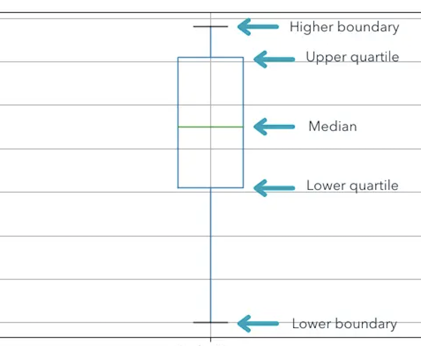
The visualization show how OPEC countries have a negative crude oil deficit, while the median sample of OECD have a positive crude oil deficit. It is also show how large economies United States (OECD member) Canada (OECD member), Saudi Arabia (OPEC member) and Russia (OEPC+ member) can influence the distributions.

Oil Refinery Load and Capacity

Extract, Transform, and Load (ETL) Data

This imports crude oil refinery utilization and capacities for countries world wide (including all OPEC members) from 1980 to 2022. A Oil Refinery processes crude oil into various refined products, including gasoline, diesel, and petrochemicals. They will be stored in the project as Pandas DataFrames, along with a third DataFrame that describes countries utilization rates of oil refineries per year.

$\text{Utilization}_{\text{year}} = \frac{\text{Refinery Throughput}_{\text{year}}}{\text{Refinery Capacity}_{\text{year}}}$

# Importing oil production dataset.
refinery_capacity_df = pd.read_csv("data/opec_downstream/world_refinery_capacity.csv", index_col="Index")
refinery_capacity_df.replace('na', np.nan, inplace=True)
refinery_capacity_df.replace('n.a.', np.nan, inplace=True)
refinery_capacity_df = refinery_capacity_df.astype(float)

# Replacing incorrectly labeled countries. 
replace = {'United States2': 'United States',
        'South Korea2': 'South Korea',
        'Venezuela3': 'Venezuela',
        'I.R.Iran2': 'I.R.Iran',
        'Qatar2': 'Qatar',
        'Saudi Arabia2': 'Saudi Arabia',
        'United Arab Emirates2': 'United Arab Emirates',
        'Algeria2': 'Algeria'
        }
refinery_capacity_df = refinery_capacity_df.rename(index=replace)

# Importing oil demand dataset. 
refinery_throughput_df = pd.read_csv("data/opec_downstream/world_refinery_throughput.csv", index_col="Index")
refinery_throughput_df.replace('na', np.nan, inplace=True)
refinery_throughput_df.replace('n.a.', np.nan, inplace=True)
refinery_throughput_df = refinery_throughput_df.astype(float)

# Merging oil production and oil demand datasets; One-to-one matching needed to compute oil deficit. 
refinery_utilization_df = refinery_capacity_df.merge(refinery_throughput_df, left_index=True, right_index=True, how='inner')

# Iterating over years of oil production and oil demand to compute oil deficit. 
for year in range(1980, 2023):
    year_x, year_y = f"{year}_x", f"{year}_y"
    refinery_utilization_df[year] = refinery_utilization_df[year_y] / refinery_utilization_df[year_x]
    refinery_utilization_df = refinery_utilization_df.drop(columns=[year_x, year_y])
    
# Fix rates for countries where throughput do not align perfectly. 
refinery_utilization_df = refinery_utilization_df.clip(upper=100)

# Transposing DataFrames to set years as index.  
refinery_capacity_df = refinery_capacity_df.transpose()
refinery_throughput_df = refinery_throughput_df.transpose()
refinery_utilization_df = refinery_utilization_df.transpose()

# Converting year index to datetime object. 
refinery_capacity_df.index = pd.to_datetime(refinery_capacity_df.index, format='%Y')
refinery_throughput_df.index = pd.to_datetime(refinery_throughput_df.index, format='%Y')
refinery_utilization_df.index = pd.to_datetime(refinery_utilization_df.index, format='%Y')

# Display. 
refinery_utilization_df.head()

Index	Algeria	Angola	Argentina	Australia	Azerbaijan	Belarus	Belgium	Brazil	Bulgaria	Canada	...	Spain	Thailand	Turkey	Turkmenistan	Ukraine	United Arab Emirates	United Kingdom	United States	Venezuela	Vietnam
1980-01-01	0.479626	0.803859	0.703216	0.786999	0.663333	0.975641	0.633019	0.778894	0.851986	0.912803	...	0.705460	0.864407	0.715847	0.669231	0.871139	0.800000	0.621653	0.781096	0.673269	NaN
1981-01-01	0.651528	0.778816	0.706140	0.736552	0.555556	0.982051	0.554717	0.752511	0.873646	0.848464	...	0.659634	0.892655	0.748634	0.669231	0.842012	0.414815	0.574662	0.747401	0.636820	NaN
1982-01-01	0.874363	0.654206	0.681287	0.753103	0.555556	0.983333	0.688705	0.729445	0.891697	0.747366	...	0.628591	0.887006	0.721030	0.597544	0.848191	0.614815	0.597545	0.748339	0.691286	NaN
1983-01-01	0.802207	0.809969	0.661743	0.696552	0.556944	0.985897	0.639118	0.705226	0.909747	0.796965	...	0.638374	0.920904	0.701717	0.597544	0.815159	0.611111	0.669634	0.730731	0.691286	NaN
1984-01-01	0.872241	0.872274	0.639586	0.701245	0.555556	0.984615	0.764415	0.749129	0.927798	0.788094	...	0.634840	0.892655	0.800429	0.597544	0.782676	0.788889	0.721209	0.776245	0.667063	NaN

5 rows × 56 columns

Because our second datasets is larger then out first dataset, we do not have perfect one-to-one matching for our third dataset. In addition here are the missing years for each country.

print('Countries in oil refinery throughput DataFrame:', len(refinery_throughput_df.columns))
print('Countries in oil refinery capacity:', len(refinery_capacity_df.columns))
print('Countries in oil refinery utilization:', len(refinery_utilization_df.columns))
refinery_utilization_df.isna().sum()

Countries in oil refinery throughput DataFrame: 76
Countries in oil refinery capacity: 56
Countries in oil refinery utilization: 56

Index
Algeria                  0
Angola                   0
Argentina                0
Australia                0
Azerbaijan               0
Belarus                  0
Belgium                  0
Brazil                   0
Bulgaria                 0
Canada                   0
Chile                    0
China                    0
Colombia                 0
Congo                    2
Croatia                  0
Ecuador                  0
Egypt                    0
France                   0
Gabon                    0
Germany                  0
I.R.Iran                 0
India                    0
Indonesia                0
Iraq                     0
Italy                    0
Japan                    0
Kazakhstan               0
Kuwait                   0
Libya                    0
Malaysia                 0
Mexico                   0
Netherlands              0
New Zealand              0
Nigeria                  0
OECD                     0
OPEC                     0
Pakistan                 0
Philippines              0
Poland                   0
Qatar                    0
Romania                  0
Russia                   0
Saudi Arabia             0
Singapore                0
South Africa             0
South Korea              0
Spain                    0
Thailand                 0
Turkey                   0
Turkmenistan             0
Ukraine                  0
United Arab Emirates     0
United Kingdom           0
United States            0
Venezuela                0
Vietnam                 14
dtype: int64

# Function plots refinery data.
def box_plot_refinery(cols, title=None):
    fig, (ax1, ax2, ax3) = plt.subplots(1, 3, figsize=(24, 8))

    # Generating x-axis labels. 
    x_labels = list(refinery_utilization_df.index.year)
    x_labels = [label if i % 5 == 0 else '' for i, label in enumerate(x_labels)]
    
    refinery_throughput_df[cols].transpose().boxplot(ax=ax1, showfliers=False)
    ax1.set_title('Total Throughput')
    ax1.set_ylabel('Crude Oil (1000 barrels/day)')
    ax1.set_xlabel('Year')

    ax1.grid(False, axis='x')
    ax1.set_xticklabels(x_labels)
    ax1.set_ylim(0, 4000)

    refinery_capacity_df[cols].transpose().boxplot(ax=ax2, showfliers=False)
    ax2.set_title('Total Capacity')
    ax2.set_ylabel('Crude Oil (1000 barrels/day)')
    ax2.set_xlabel('Year')
    ax2.grid(False, axis='x')
    ax2.set_xticklabels(x_labels)
    ax2.set_ylim(0, 4000)

    refinery_utilization_df[cols].transpose().boxplot(ax=ax3, showfliers=False)  
    ax3.set_title('Utilization')
    ax3.set_ylabel('Rate (%)')
    ax3.set_xlabel('Year')
    ax3.grid(False, axis='x')
    ax3.set_xticklabels(x_labels)
    ax3.set_ylim(0, 1)


    fig.suptitle(title, fontsize=20, y=1.02)
    plt.tight_layout()

opec_sample_countries = opec_countries[opec_countries.isin(refinery_utilization_df.columns)]
box_plot_refinery(opec_sample_countries, title="Sample OPEC Countries Oil Refinery Metrics")

oecd_sample_countries = oecd_countries[oecd_countries.isin(refinery_utilization_df.columns)]
box_plot_refinery(oecd_sample_countries, title="Sample OECD Countries Oil Refinery Metrics")

OPEC Countries have more variance is their utilization of oil refineries then OECD countries. A factor of this could be the fact that OPEC sets production quotas for member countries, forcing members to not produce and use oil refineries at the most optimal domestic rate.

Crude Oil Spot Prices

Extract, Transform, and Load (ETL) Data

This imports crude oil spot prices for countries world wide (including all OPEC members) from 1983 to 2022. The Spot Price is the current market equilibrium of a future contract; this is used to determine the current price a future contracts, which is how oil is traded.

# Importing oil spot price dataset. 
oil_spot_prices_df = pd.read_csv("data/opec_prices/oil_spot_prices.csv", index_col="Index")
oil_spot_prices_df.replace('na', np.nan, inplace=True)
oil_spot_prices_df = oil_spot_prices_df.astype(float)

# Creating 2D index for countries with multiple oil benchmarks.  
oil_spot_prices_df.index = oil_spot_prices_df.index.str.split(' - ', expand=True)

# Replacing incorrectly labeled countries. 
oil_spot_prices_df = oil_spot_prices_df.rename(index={'IR Iran': 'I.R.Iran'})

# Transposing DataFrames to set years as index.  
oil_spot_prices_df = oil_spot_prices_df.transpose()

# Convert the index to datetime
oil_spot_prices_df.index = pd.to_datetime(oil_spot_prices_df.index, format='%Y')

# Display.
oil_spot_prices_df.head()

	Algeria	Angola	Egypt	I.R.Iran	Indonesia	Libya	Malaysia		Mexico		...	Norway	Oman	Qatar	Russia	Saudi Arabia	United Kingdom		United States	United Arab Emirates	OPEC
	Zarzaitine	Cabinda	Suez Mix	Iran Light	Minas	Brega	Miri	Tapis	Isthmus	Maya	...	Oseberg	Oman	Dukhan	Urals	Arab Heavy	BrentDated	Forties	WTI	Dubai	ORB
1983-01-01	30.398	NaN	NaN	28.145	28.981	29.740	NaN	NaN	28.817	NaN	...	NaN	28.748	29.122	NaN	26.590	29.715	29.572	30.413	28.180	29.037
1984-01-01	29.087	NaN	27.197	26.810	27.962	28.879	NaN	NaN	28.192	NaN	...	NaN	28.019	28.018	NaN	26.681	28.715	28.586	29.393	27.522	28.204
1985-01-01	27.925	NaN	25.870	26.034	25.990	27.789	NaN	NaN	26.858	NaN	...	NaN	26.944	27.150	NaN	25.833	27.533	27.472	27.960	26.491	27.007
1986-01-01	14.832	NaN	12.619	13.501	13.415	14.313	NaN	NaN	13.433	NaN	...	NaN	13.288	13.458	NaN	NaN	14.274	14.182	14.913	12.956	13.533
1987-01-01	18.095	NaN	16.748	17.027	17.779	17.675	NaN	NaN	17.809	15.261	...	NaN	17.252	17.395	17.289	16.083	18.406	18.270	19.164	16.916	17.725

5 rows × 22 columns

Here are the missing years for each country and benchmark.

oil_spot_prices_df.isna().sum()

Algeria               Zarzaitine    0
Angola                Cabinda       9
Egypt                 Suez Mix      1
I.R.Iran              Iran Light    0
Indonesia             Minas         0
Libya                 Brega         0
Malaysia              Miri          8
                      Tapis         7
Mexico                Isthmus       0
                      Maya          4
Nigeria               Forcados      0
Norway                Ekofisk       0
                      Oseberg       8
Oman                  Oman          0
Qatar                 Dukhan        0
Russia                Urals         4
Saudi Arabia          Arab Heavy    1
United Kingdom        BrentDated    0
                      Forties       0
United States         WTI           0
United Arab Emirates  Dubai         0
OPEC                  ORB           0
dtype: int64

Exploratory Data Analysis (EDA)

Oil spot prices are categorized by country and benchmark, such that countries can have multiple benchmarks or tack each others. Too analize how spot price benchmarks vary from each other, I normalize the spot prices using the Z-Score then compute a 5-year moving average. This is done for OPEC and OECD countries where spot price data was available.

# Function plots the spot prices of oil, z-score dist. of spot prices and the 10 year moving average of z-score dist. for given list of countries. 
def line_plot_price(cols, title):
    fig, (ax1, ax2, ax3) = plt.subplots(1, 3, figsize=(24, 8))

    oil_spot_prices_df[cols].plot(kind='line', legend=False, ax=ax1)
    ax1.set_xlabel('Year')
    ax1.set_ylabel('Crude Oil (1000 barrels/day)')
    ax1.set_title('Spot Prices')
    ax3.axhline(y=0, color='black', linestyle='--')

    # Computing the z-score
    oil_spot_prices_norm = oil_spot_prices_df[cols].apply(zscore, axis=1)

    oil_spot_prices_norm.plot(kind='line', legend=False, ax=ax2)
    ax2.set_xlabel('Year')
    ax2.set_ylabel('Spot Price (Z-Score)')
    ax2.set_title('Normalized Spot Prices')
    ax3.axhline(y=0, color='black', linestyle='--')

    # Computing moving average for normalized spot prices.   
    oil_spot_prices_ma = oil_spot_prices_norm.rolling(window=5, min_periods=5).mean()

    oil_spot_prices_ma.plot(kind='line', legend=False, ax=ax3)
    ax3.set_xlabel('Year')
    ax3.set_ylabel('Spot Price (Z-Score)')
    ax3.set_title('Normalized 5-Year Moving Average Spot Prices ')
    ax3.axhline(y=0, color='black', linestyle='--')

    lines, labels = ax1.get_legend_handles_labels()
    fig.legend(lines, labels, loc='center', bbox_to_anchor=(0.5, -0.1), ncol=3)
    fig.suptitle(title, fontsize=20, y=1.02)
    plt.tight_layout()
    

oil_spot_prices_countries = tuple(zip(*oil_spot_prices_df))[0]
opec_sample_countries = opec_countries[opec_countries.isin(oil_spot_prices_countries)]
line_plot_price(opec_sample_countries, "Sample OPEC Spot Prices by Country and Benchmark")

oecd_sample_countries = oecd_countries[oecd_countries.isin(oil_spot_prices_countries)]
line_plot_price(oecd_sample_countries, "Sample OECD Spot Prices by Country and Benchmark")

Observations from the spot price visualizations:

• Saudi Heavy oil trades as a discount relative to all OPEC countries.
• WIT oil became relatively cheaper then other OECD countries between 2003 and 2013.
• The United Kingdoms Brent and Forties benchmarks trade at a tight spread from eachother. A factor of this is because Brent is a composite of the Forties benchmark.

OPEC Crude Oil Production Quotas

OPEC quotas are production limits established for its member countries to regulate the global supply of oil; acting as a cartel supplier in economics. These quotas are set during OPEC meetings, where member nations agree on individual production targets and requires trusting member countries. Historically, due to geopolitical conflict and economic collapse, member countries consistently underproduce and overproduce targets.

Extract, Transform, and Load (ETL) Data

# Importing oil spot price dataset. 
oil_targets_df = pd.read_csv("data/summary/crude_oil_target.csv", index_col='Index')

def extract_numbers(s):
    numeric_values = re.findall(r'\d+', str(s))
    if numeric_values:
        return float(str().join(numeric_values))
    else:
        return np.NaN

oil_targets_df = oil_targets_df.applymap(extract_numbers)

# Transposing DataFrames to set years as index.  
oil_targets_df = oil_targets_df.transpose()

# Replacing incorrectly labeled countries. 
oil_targets_df = oil_targets_df.rename(columns={'IR Iran': 'I.R.Iran'})

# Removing sub exemptions from the quota values.  
opec_targets = ['OPEC', 'OPEC excl Iraq', 'OPEC excl Angola and Iraq',]
oil_targets_df[opec_targets] = oil_targets_df[opec_targets].apply(pd.to_numeric, errors='coerce')

# Converting date ranges to date time objects. 
oil_targets_df.index =  oil_targets_df.index.map(lambda x: x[:5])
oil_targets_df.index =  pd.to_datetime(oil_targets_df.index, format='%b%y')

# Dropping errors in the data. 
oil_targets_df.drop(['1998-04-01', '2006-11-01', '2007-02-01', '2008-11-01'], inplace=True)

# Display.
print(oil_targets_df.shape)
oil_targets_df.tail()

(75, 16)

Index	Algeria	Angola	Congo	Equatorial Guinea	Gabon	I.R.Iran	Iraq	Kuwait	Libya	Nigeria	Saudi Arabia	United Arab Emirates	Venezuela	OPEC	OPEC excl Iraq	OPEC excl Angola and Iraq
2022-07-01	1039.0	1502.0	320.0	125.0	183.0	NaN	4580.0	2768.0	NaN	1799.0	10833.0	3127.0	NaN	26276.0	NaN	NaN
2022-08-01	1055.0	1525.0	325.0	127.0	186.0	NaN	4651.0	2811.0	NaN	1826.0	11004.0	3179.0	NaN	26689.0	NaN	NaN
2022-09-01	1057.0	1529.0	325.0	127.0	187.0	NaN	4663.0	2818.0	NaN	1830.0	11030.0	3186.0	NaN	26752.0	NaN	NaN
2022-10-01	1055.0	1525.0	325.0	127.0	186.0	NaN	4651.0	2811.0	NaN	1826.0	11004.0	3179.0	NaN	26689.0	NaN	NaN
2022-11-01	1007.0	1455.0	310.0	121.0	177.0	NaN	4431.0	2676.0	NaN	1742.0	10478.0	3019.0	NaN	25416.0	NaN	NaN

Because OPEC meetings do not happen at scheduled times, we have to transform the quota data into annual sums.

# Converting monthly quota data to be summed by year.
date_range = pd.date_range(start='1983-01-01', end='2021-12-01', freq='MS')
temp_oil_targets_df = pd.DataFrame(columns=oil_targets_df.columns)
i = 0

for date in date_range:    
    row = oil_targets_df.iloc[i]
    next_row = oil_targets_df.iloc[i+1]
    
    if date < next_row.name:
        row.name = date
        temp_oil_targets_df = temp_oil_targets_df.append(row, ignore_index=False)
    else:
        next_row.name = date
        temp_oil_targets_df = temp_oil_targets_df.append(next_row, ignore_index=False)
        i += 1
    
def sum(series):
    if any(pd.isna(series)):
        return np.NaN
    else:
        return np.sum(series) / 12

temp_oil_targets_df = temp_oil_targets_df.groupby(pd.Grouper(freq='Y'))
temp_oil_targets_df = temp_oil_targets_df.agg(sum)
temp_oil_targets_df.index = pd.to_datetime(temp_oil_targets_df.index.year, format='%Y')
temp_oil_targets_df.head()

Index	Algeria	Angola	Congo	Equatorial Guinea	Gabon	I.R.Iran	Iraq	Kuwait	Libya	Nigeria	Saudi Arabia	United Arab Emirates	Venezuela	OPEC	OPEC excl Iraq	OPEC excl Angola and Iraq
1983-01-01	706.250000	NaN	NaN	NaN	150.000000	2100.000000	1200.0	987.5	1012.500000	1300.000000	5537.500000	1075.0	1631.250000	15700.000000	NaN	NaN
1984-01-01	714.666667	NaN	NaN	NaN	147.833333	2383.333333	1200.0	1025.0	1081.666667	1300.000000	4892.166667	1075.0	1655.000000	15474.666667	NaN	NaN
1985-01-01	663.000000	NaN	NaN	NaN	137.000000	2300.000000	1200.0	900.0	990.000000	1300.000000	4353.000000	950.0	1555.000000	14348.000000	NaN	NaN
1986-01-01	664.000000	NaN	NaN	NaN	140.833333	2302.833333	NaN	910.0	991.500000	1300.666667	4353.000000	950.0	1558.166667	NaN	NaN	NaN
1987-01-01	651.000000	NaN	NaN	NaN	155.500000	2312.000000	1503.0	972.0	972.000000	1269.500000	4238.000000	925.0	1533.000000	14531.000000	NaN	NaN

oil_targets_df.isna().sum()

Index
Algeria                       7
Angola                       48
Congo                        50
Equatorial Guinea            49
Gabon                        29
I.R.Iran                     33
Iraq                         31
Kuwait                        8
Libya                        34
Nigeria                       9
Saudi Arabia                  7
United Arab Emirates          7
Venezuela                    32
OPEC                         29
OPEC excl Iraq               51
OPEC excl Angola and Iraq    74
dtype: int64

Exploratory Data Analysis (EDA)

There is a lot of missing values in our transformed dataset. Considering this, we will only plot the two nations with the most data available: Saudi Arabia and the United Arab Emirates.

# Plotting nations quotas and production. 
def plot_quotas(countries):
    fig, axs = plt.subplots(len(countries), 1, figsize=(12, 6*len(countries)))
    for i, country in enumerate(countries):
        axs[i].plot(oil_targets_df.index, oil_targets_df[country], color='blue', label='OPEC Quota')
        axs[i].plot(oil_production_df.index, oil_production_df[country], color='red', label='Production')
        axs[i].set_title(f"{country}'s Crude Oil OPEC Quota and Production Over Time")
        axs[i].set_xlabel('Year')
        axs[i].set_ylabel('Crude Oil (1000 barrels/day)')
        axs[i].legend()

plot_quotas(['Saudi Arabia', 'United Arab Emirates'])

Model: Random Forest Regression of Overproduction

Before model training, I note the following data errors and observations based on ETL:

1. All nations produce a negative deficit (positive surplus) of crude oil.
2. Some nations have over 100% utilization rate; this could be an error in my feature engineering.
3. The majority of OPEC nations are missing over 50% of their quota data; excluding the UAE and Saudi Arabia.

Having tested LinearRegression, PolynomialFeatures, DecisionTree and RandomForest regression models. I discovered that a RandomForest regression model produces the best test accuracy.

Assumptions followed for RandomForest regression model:

1. There little to zero autocorrelation (correlation over time) in the dataset.
2. Calculation of production quota by year is correct.
3. All input features are continuous features.

The regression model will Predict the overproduction of OPEC nation crude oil. The dependent variable being percentage of overproduction with independent variables being, refinery throughput, domestic demand and spot price premium (premium above OPEC Oil Reference Basket). The training and test dataset will only be a combination of annual observations from Saudi Arabia and the United Arab Emirates, this is because these two nation are the largest crude oil producers in OPEC and is the only data that exists across all six ETL datasets.

Letting overproduction be a percentage:

$\text{Overproduction}_{\text{year}} =\frac{ \text{Target}_{\text{year}} - \text{Production}_{\text{year}}}{\text{Production}_{\text{year}}}$

The regression model is defined as:

$\hat{Overproduction}_{\text{year}} = \frac{1}{100} \sum_{i=1}^{100} h_i(x)$

$100 := Number of Decision Trees$

$h_i(x):= Decision Tree Prediction$

By creating this model, it is also be determined what features inputs were most influential in predicting overproduction.

Combining Datasets for Machine Learning

# Combining all time interval data for a single OPEC nation. 
def merge_opec_datasets(country): 
    columns = [
        oil_production_df[country].rename('production'),
        oil_demand_df[country].rename('demand'),
        refinery_capacity_df[country].rename('capacity'),
        refinery_throughput_df[country].rename('throughput'),
        oil_spot_prices_df[country].iloc[:, 0].rename('price'),
        temp_oil_targets_df[country].rename('target'),
        ]
    
    # Combining datasets. 
    df = pd.concat(columns, axis=1)
    
    # Adding two new features. 
    df['premium'] = (df['price'] - oil_spot_prices_df['OPEC']['ORB']) / oil_spot_prices_df['OPEC']['ORB']
    df['overproduction'] = (df['production'] - df['target']) / df['target']
    
    df = df[(df.index >= '1983-01-01') & (df.index <= '2021-01-01')]

    # Filling np.NaNs for ML. 
    df = df.dropna(subset=['overproduction'])
    imputer = SimpleImputer(strategy='median') 
    df = pd.DataFrame(imputer.fit_transform(df), columns=df.columns)   
    return df

# Combining all time interval data for a multiple OPEC nation. 
def merge_opec_countries(countries):
    dfs = list()
    
    for country in countries:
        try:
            df = merge_opec_datasets(country)   
            dfs.append(df)
            
        except KeyError as error: 
            print(f"{error} does not exist across all datasets.")    
            
    df = pd.concat(dfs, axis=0)
    
    return df

df = merge_opec_countries(['Saudi Arabia', 'United Arab Emirates'])
print(df.shape)
df.head()

(54, 8)

	production	demand	capacity	throughput	price	target	premium	overproduction
0	4539.410	835.0	935.0	851.0	26.5900	5537.500000	-0.084272	-0.180242
1	4079.081	936.0	1190.0	855.0	26.6810	4892.166667	-0.053999	-0.166202
2	3174.955	992.0	1440.0	1015.0	25.8330	4353.000000	-0.043470	-0.270628
3	4784.200	941.0	1440.0	1096.0	24.3145	4353.000000	-0.078211	0.099058
4	3975.150	899.0	1425.0	1337.0	16.0830	4238.000000	-0.092638	-0.062022

Correlation and Shape of Dataset

# Corr Matrix
corr = df.corr()
corr.style.background_gradient(cmap='coolwarm')

	production	demand	capacity	throughput	price	target	premium	overproduction
production	1.000000	0.873565	0.924768	0.943318	0.227779	0.993033	-0.288670	-0.256592
demand	0.873565	1.000000	0.942345	0.930889	0.518721	0.883269	0.067248	-0.275140
capacity	0.924768	0.942345	1.000000	0.989762	0.437776	0.928178	-0.081870	-0.315857
throughput	0.943318	0.930889	0.989762	1.000000	0.419847	0.941562	-0.131174	-0.292931
price	0.227779	0.518721	0.437776	0.419847	1.000000	0.242529	0.562840	-0.211642
target	0.993033	0.883269	0.928178	0.941562	0.242529	1.000000	-0.246618	-0.342494
premium	-0.288670	0.067248	-0.081870	-0.131174	0.562840	-0.246618	1.000000	-0.219329
overproduction	-0.256592	-0.275140	-0.315857	-0.292931	-0.211642	-0.342494	-0.219329	1.000000

fig, axs = plt.subplots(figsize=(18, 18))
scatter_matrix(df, alpha=0.7, s=100, diagonal='kde', ax=axs)
fig.suptitle(f"Matrix Scatter Plot of Features", fontsize=20)
fig.tight_layout()

/var/folders/rq/9zvkr67d2mx07n6md37__xcr0000gn/T/ipykernel_4420/766286048.py:2: UserWarning: To output multiple subplots, the figure containing the passed axes is being cleared.
  scatter_matrix(df, alpha=0.7, s=100, diagonal='kde', ax=axs)

Training Random Forest Model

Based on the correlation plots, it appears that domestic demand, refinery capacity and premium have the lowest correlation across the feature space. These three features will be the input used to predict the hypothesis space.

Input descriptions:

1. demand: A OPEC nations domestic demand for crude oil.
2. throughput: The amount of crude oil refined into final products domestically by an OPEC nation.
3. premium: The percentage a nations crude oil spot price is above (or below) the OPEC Oil Reference Basket.

# Splitting features.
X, y = df.drop(columns=['production', 'target', 'overproduction', 'price', 'capacity']), df['overproduction']

# Separating train and test. 
X_train, X_test, y_train, y_test = train_test_split(X, y, test_size=0.3, random_state=42)

print("X Train Shape:", X_train.shape)
print("X Test Shape:", X_test.shape)
    
# Fit linear polynomial regression model. 
model = RandomForestRegressor(random_state=42, n_estimators=100)
model.fit(X_train, y_train)

X Train Shape: (37, 3)
X Test Shape: (17, 3)

RandomForestRegressor(random_state=42)

In a Jupyter environment, please rerun this cell to show the HTML representation or trust the notebook.
On GitHub, the HTML representation is unable to render, please try loading this page with nbviewer.org.

Measuring the Model's Accuracy

Because the model is predicting a percentage value, accuracy will be measured using Mean Absolute Error. This way our model output and error are both percentage values.

$\text{MAE} = \frac{1}{n} \sum_{i=1}^{n} |Overproduction_i - \hat{Overproduction}_i|$

fig, axs = plt.subplots(1, 2, figsize=(16, 8))

# Testing model accuracy. 
y_pred_test = model.predict(X_test)
residuals_test = y_test - y_pred_test
mae_test = mean_absolute_error(y_test, y_pred_test)    

axs[0].scatter(y_test , residuals_test, alpha=0.7, s=50)
axs[0].axhline(y=0, color='r', linestyle='-', linewidth=2) 
axs[0].set_title(f'Test Data Residual Errors\nmean_absolute_error = {mae_test:.2f} | mean percentage = {y_test.mean():.2f}')
axs[0].set_xlabel('Actual Value (%)')
axs[0].set_ylabel('Residual Error (%)')

# Model accuracy for training set. 
y_pred_train = model.predict(X_train)
residuals_train = y_train - y_pred_train
mae_train = mean_absolute_error(y_train, y_pred_train) 

axs[1].scatter(y_train , residuals_train, alpha=0.7, s=50)
axs[1].axhline(y=0, color='r', linestyle='-', linewidth=2)
axs[1].set_title(f'Train Data Residual Errors\nmean_absolute_error = {mae_train:.2f} | mean percentage = {y_train.mean():.2f}')
axs[1].set_xlabel('Actual Value (%)')
axs[1].set_ylabel('Residual Error (%)')

Text(0, 0.5, 'Residual Error (%)')

This model is not significantly accurate at predicting the overproduction percentage. To simplify the measure of accuracy, lets measure the models precision at correctly predicting positive overproduction value.

test = list(map(lambda x: x > 0, y_test))
pred = list(map(lambda x: x > 0, y_pred_test))
precision = precision_score(test, pred)
recall = recall_score(test, pred)
print("Overproduction Model Precision:", precision)
print("Overproduction Model Recall:", recall)

Overproduction Model Precision: 0.7272727272727273
Overproduction Model Recall: 0.6666666666666666

The model is more precise at correctly predicting when overproduction occurs.

Determining Feature Importance

Finally, the model can used to infer what features are the most important for predicting overproduction.

importances = dict(zip(X.columns, model.feature_importances_))
print("Features importance in model:")
for feature, importance in importances.items():
    print(f"    {feature}: {importance:.2f}")

Features importance in model:
    demand: 0.32
    throughput: 0.34
    premium: 0.34

This shows that features selected ended up having nearly equal importance in fitting the model. With each feature holding approximately one third of weight in the model.

# Converting python notebook to html.
!jupyter nbconvert --to html final.ipynb --output index

[NbConvertApp] Converting notebook final.ipynb to html
[NbConvertApp] Writing 2187671 bytes to index.html